Data Structure Chapter 1 & 2

Introduction to

Algorithm

What is an Algorithm? (1/2) 
• Definition

– A computable set of steps to achieve a desired result
What is an Algorithm? (2/2) 
• Properties

      –  Finiteness -> an algorithm terminates after a finite numbers of steps 


      –  Definiteness -> each step in algorithm is unambiguous. This means that the action specified by the step cannot be interpreted (explain the meaning of) in multiple ways & can be performed without any confusion 


      –  Input -> an algorithm accepts zero or more inputs 


      –  Output -> it produces at least one output 


      –  Effectiveness -> it consists of basic instructions that are realizable. This means that the instructions can be performed by using the given inputs in a finite amount of time 


Classes of Algorithm (1/4)

• There is no universally accepted breakdown for the various types of algorithms, but there are common classes that algorithms are frequently agreed to belong to e.g.

• Dynamic Programming Algorithms: This class remembers older results and attempts to use this to speed the process of finding new results.

Classes of Algorithm (2/4)

• Greedy Algorithms: Greedy algorithms attempt not only to find a solution, but to find the ideal solution to any given problem.

• Brute Force Algorithms: The brute force approach starts at some random point and iterates through every possibility until it finds the solution.

• Randomized Algorithms: This class includes

any algorithm that uses a random number at

any point during its process.

Classes of Algorithm (3/4)

• Branch and Bound Algorithms: Branch and bound algorithms form a tree of subproblems to the primary problem, following each branch until it is either solved or lumped in with another branch.

• Simple Recursive Algorithms: This type of algorithm goes for a direct solution immediately, then backtracks to find a simpler solution.

Classes of Algorithm (4/4)

• Backtracking Algorithms: Backtracking algorithms test for a solution, if one is found the algorithm has solved, if not it recurs once and tests again, continuing until a solution is found.

• Divide and Conquer Algorithms: A divide and conquer algorithm is similar to a branch and bound algorithm, except it uses the backtracking method of recurring in tandem with dividing a problem into subproblems.

Algorithm Analysis (1/15) • Why should we analyze algorithms?

– A problem may have numerous algorithmic solutions.

– In order to choose the best algorithm for a particular task, you need to be able to judge how long a particular solution will take to run.

– Or, more accurately, you need to be able to judge how long two solutions will take to run, and choose the better of the two.

– You don't need to know how many minutes and seconds they will take, but you do need some way to compare algorithms against one another.

Algorithm Analysis (2/15)

• Most algorithms transform input objects into output objects.

• The running time of an algorithm typically grows with the input size.

• Average case time is often difficult to determine.

• We focus on the worst case running time.

– Easier to analyze

– Crucial to applications such as games, finance and robotics

Algorithm Analysis (3/15)

• How to Calculate Running Time

– Write a program implementing the algorithm

– Run the program with inputs of varying size and composition

– Use a method like System.currentTimeMillis() to get an accurate measure of the actual running time

– Plot the results

Algorithm Analysis (4/15) 
• Limitations

– It is necessary to implement the algorithm, which may be difficult.

– Results may not be indicative of the running time on other inputs not included in the experiment.

– In order to compare two algorithms, the same hardware and software environments must be used.

Algorithm Analysis (5/15) 
• Theoretical Analysis

– Uses a high-level description of the algorithm instead of an implementation

– Characterizes running time as a function of the input size, n.

– Takes into account all possible inputs

– Allows us to evaluate the speed of an algorithm independent of the hardware/software environment

Algorithm Analysis (6/15)

• Primitive Operations

– Basic computations performed by an algorithm

– Identifiable in pseudocode

– Largely independent from the programming language

– Exact definition not important (we will see why later)

– Assumed to take a constant amount of time in the RAM model

Algorithm Analysis (7/15)

• Primitive Operations Examples: – Evaluating an expression
– Assigning a value to a variable
– Indexing into an array

– Calling a method
– Returning from a method

Algorithm Analysis (8/15) 
• Counting Primitive Operations

• By inspecting the pseudocode, we can

determine the maximum number of primitive

operations executed by an algorithm, as a

function of the input size

Algorithm arrayMax(A, n) currentMax ¬ A[0]
for i ¬ 1 to n - 1 do
if A[i] > currentMax then currentMax ¬ A[i]

{ increment counter i } return currentMax

# operations 1

n
(n - 1) (n - 1) (n - 1) 1
4n - 1

Total

Algorithm Analysis (9/15) 
• Estimating Running Time

– Algorithm arrayMax executes 4n - 1 primitive operations in the worst case.

– Define:

• a = Time taken by the fastest primitive operation 
• b = Time taken by the slowest primitive operation

– Let T(n) be worst-case time of arrayMax. Then • a(4n-1)<=T(n)<=b(4n-1)

– Hence, the running time T(n) is bounded by two linear functions

Algorithm Analysis (10/15) 
• Growth Rate Vs Running Time

– Changing the hardware/ software environment 
• Affects T(n) by a constant factor, but
• Does not alter the growth rate of T(n)

– The linear growth rate of the running time T(n) is an intrinsic property of algorithm arrayMax

Algorithm Analysis (11/15)

•  Worst-case Complexity

            –  Maximum steps the algorithm takes for any possible input. 


            –  Most tractable measure. 


•  Average-case Complexity

            –  Average of the running times of all possible inputs. 


            –  Demands a definition of probability of each input, 
which is usually difficult to provide and to analyze. 


•  Best-case Complexity 
– Minimum number of steps for any possible input. – Not a useful measure. 


Algorithm Analysis: (12/15) 
Example

Alg.: MIN (a[1], ..., a[n]) m ← a[1];

for i ← 2 to n if a[i] < m

then m ← a[i]; Running time:

– the number of primitive operations (steps)

executed before termination
T(n) =1 [first step] + (n) [for loop] + (n-1) [if condition] + (n-1) [the assignment in then] = 3n - 1

Order (rate) of growth:

– The leading term of the formula

– Expressestheasymptoticbehaviorofthealgorithm


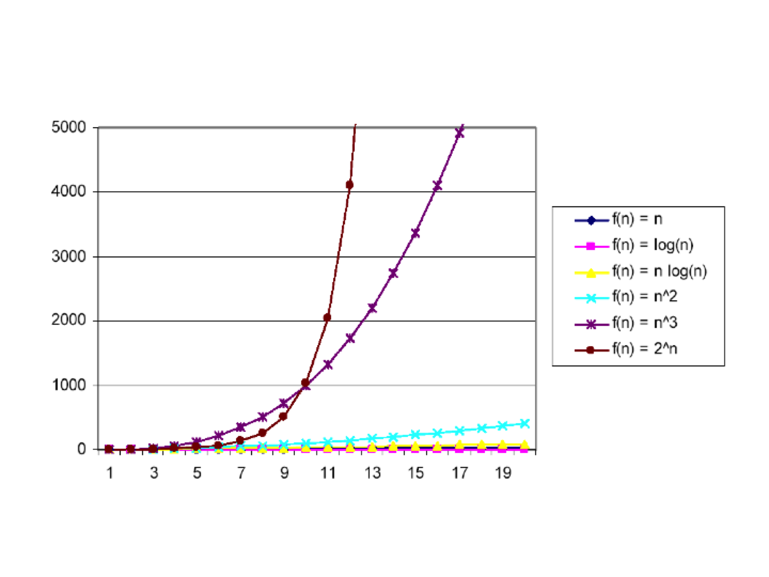
Algorithm Analysis: (13/15) • Typical Running Time Functions

– 1 (constant running time):
• Instructions are executed once or a few times

– logN (logarithmic)
• A big problem is solved by cutting the original problem in smaller

sizes, by a constant fraction at each step – N (linear)

• A small amount of processing is done on each input element – N logN

• A problem is solved by dividing it into smaller problems, solving them independently and combining the solution

Algorithm Analysis: (14/15) • Typical Running Time Functions

– N2 (quadratic)
• Typical for algorithms that process all pairs of data items (double

nested loops) – N3 (cubic)

• Processing of triples of data (triple nested loops)

– NK (polynomial)

– 2N (exponential)
• Few exponential algorithms are appropriate for practical use

Algorithm Analysis: (15/15)

•

Asymptotic Notations

A way to describe behavior of functions in the limit – Abstracts away low-order terms and constant factors
– How we indicate running times of algorithms
– Describe the running time of an algorithm as n grows to ¥

• • •

O notation: (Big Oh)
– asymptotic “less than”:

W notation: (Big Omega) – asymptotic “greater than”:

Q notation: (Big Theta) – asymptotic “equality”:

f(n) “≤” g(n) f(n) “≥” g(n) f(n) “=” g(n)

O(Big Oh) -Notation

O(Big Oh) - Example

•  2n2 = O(n3): 


•  1000n2+1000n = O(n2): 


2n2 ≤cn3Þ2≤cnÞc=1andn0=2 • n2 = O(n2): n2 ≤ cn2 Þ c ≥ 1 Þ c = 1 and n0= 1

1000n2+1000n ≤ 1000n2+ 1000n2 = 2000n2
Þ c=2000 and n0 = 1

•  n = O(n2): n ≤ cn2 Þ cn ≥ 1 Þ c = 1 and n0= 1 


•  2n + 10 = O(n) : 


•  n2¹O(n) 


•  7n -2 = O(n) 


•  3n3 + 20n2 + 5 = O(n3) 


•  3 logn + log log n = O(log n) 


W (Big Omega) - Notation

• Intuitively: W(g(n)) = the set of functions with a larger or same order of growth as g(n)

W (Big Omega) - Example – 5n2 = W(n)

$ c, n0 such that: 0 £ cn £ 5n2 Þ cn £ 5n2 – 100n + 5 ≠ W(n2)

$c,n0 suchthat:0£cn2 £100n+5 100n + 5 £ 100n + 5n (" n ³ 1) = 105n

cn2 £ 105n
Since n is positive Þ cn – 105 £ 0

Þ c = 1 and n0 = 1

Þ n(cn – 105) £ 0
Þ contradiction: n cannot be smaller than a constant

– n = W(2n), n3 = W(n2), n = W(logn)


Þ n £ 105/c

Q (Big Theta) - Notation

• Intuitively Q(g(n)) = the set of functions with the same order of growth as g(n)

Q (Big Theta) - Example • n2/2 –n/2 = Q(n2)

•  1⁄2 n2 - 1⁄2 n ≤ 1⁄2 n2 "n ≥ 0 Þ c2= 1⁄2 


•  1⁄2 n2 - 1⁄2 n ≥ 1⁄2 n2 - 1⁄2 n * 1⁄2 n ( "n ≥ 2 ) = 1⁄4 n2 Þ c1= 1⁄4 
– n≠Q(n2):c1 n2 ≤n≤c2 n2 Þ only holds for: n ≤ 1/c1 
6n3 ≠ Q(n2):c1 n2 ≤6n3 ≤c2 n2 Þ only holds for: n ≤ c2 /6 
n≠Q(logn):c1 logn≤n≤c2 logn
Þ c2 ≥ n/logn, " n≥ n0 – impossible 


Asymptotic Notations - Exercise

• For each of the following pairs of functions, either f(n) is O(g(n)), f(n) is Ω(g(n)), or f(n) is Θ(g(n)). Determine which relationship is correct.

      –  f(n) = log n2; g(n) = log n + 5 


      –  f(n) = n; g(n) = log n2 


      –  f(n) = log log n; g(n) = log n 


      –  f(n) = n; g(n) = log2 n 


      –  f(n) = n log n + n; g(n) = log n 


      –  f(n) = 10; g(n) = log 10 


      –  f(n) = 2n; g(n) = 10n2 


      –  f(n) = 2n; g(n) = 3n 


f(n) = Q (g(n)) f(n) = W(g(n)) f(n) = O(g(n)) f(n) = W(g(n)) f(n) = W(g(n)) f(n) = Q(g(n)) f(n) = W(g(n)) f(n) = O(g(n))

More on Asymptotic Notations

•  There is no unique set of values for n0 and c in proving the asymptotic bounds 


•  Prove that 100n + 5 = O(n2)
– 100n+5≤100n+n=101n≤101n2 
for all n ≥ 5
n0 =5andc=101isasolution 
– 100n+5≤100n+5n=105n≤105n2 for all n ≥ 1 


n0 = 1 and c = 105 is also a solution
Must find SOME constants c and n0 that satisfy the asymptotic notation relation

Comparisons of Functions

•  Theorem:
f(n) = Q(g(n)) Û f = O(g(n)) and f = W(g(n)) 


•  Transitivity:
– f(n) = Q(g(n)) and g(n) = Q(h(n)) Þ f(n) = Q(h(n)) 
– SameforOandW 


•  Reflexivity: 
– f(n) = Q(f(n)) 
– SameforOandW 


•  Symmetry: 
– f(n) = Q(g(n)) if and only if g(n) = Q(f(n)) 


•  Transpose symmetry: 
– f(n) = O(g(n)) if and only if g(n) = W(f(n))
 


•

Asymptotic Notations in Equations

On the right-hand side
– Q(n2) stands for some anonymous function in Q(n2) 2n2 + 3n + 1 = 2n2 + Q(n) means:
There exists a function f(n) Î Q(n) such that

2n2 + 3n + 1 = 2n2 + f(n)

On the left-hand side

2n2 + Q(n) = Q(n2)

No matter how the anonymous function is chosen on the left-hand side, there is a way to choose the anonymous function on the right-hand side to make the equation valid.

Sorting Algorithms

Name	Best	Average	Worst	Method
Quick	n log n	n log n	n2	Partitioning
Merge	n log n	n log n	n log n	Merging
Heap	n log n	n log n	n log n	Selection
Insertion	n	n2	n2	Insertion
Selection	n2	n2	n2	Selection
Bubble	n2	n2	n2	Exchanging

Other Sorting Algorithms

• Introsort
• Timsort
• Shell sort
• Binary Tree sort • Cycle sort

• Library sort
• Patience sort • Smoothsort

• Strand sort • Tournament

sort
• Cocktail sort • Comb sort
• Gnome sort • Bogosort

Comparison Sort

Other Sorting Algorithms

• Pigeonhole sort • Bucket sort
• Counting sort
• LSD Radix sort
• MSD Radix sort • Spreadsort

Non Comparison Sort

______________________________________________________________________________________

Introduction to Data Structures 

• Problem solving =

– Understanding the problem – Designing a solution

– Implementing the solution 

• What exactly is a solution? – A solution = a program 

An Algorithm 

• An algorithm is a sequence of steps that take us from the input to the output.

• Properties of Algorithm 

–  Input: may or may not some input data

–  Output: at least one output

–  Definiteness: every step must be clear and unambiguous

–  Finiteness: It must terminate after a finite number of steps

–  Effectiveness: the steps must be basic steps so that dry-run will be possible

Data Organization 

• Any algorithm we come up with will have to manipulate data in some way 

– The way we choose to organize our data directly affects the efficiency of our algorithm 

• Solution = algorithm + data organization

– Both components are strongly interconnected. 

Data structures 

• Data structure: An arrangement of data in a computer’s memory (or sometimes on a disk).

• conceptual and concrete ways to organize data for efficient storage and efficient manipulation 

– Arrays, linked lists, stacks, trees, hash tables. 

• Algorithms manipulate the data in these 

structures in order to accomplish some task. – Inserting an item, search for an item, sorting. 

How are Data structures used • As an actual way to store real-world data 

– e.g., lists, trees

• As a tool to be used only within a program 

(not visible to the user)

– E.g., stacks, queues, priority queues 

• As a model of real-world situations – e.g., graphs 

Why different data structures 

• Each data structure has different advantages and disadvantages, and will be useful for different types of applications. 

– Example: arrays

• Fast access: if we know the index of the item we are looking for • Insertion and Deletion is slow

• size is fixed 

– Maintain a Job Queue • Queuecanbeused 

– Hierarchy of employees of an organization • Tree can be used  

Stack 

Types of data structures 

Data Structure 

Linear Non Linear 

Queue Tree Graph 

ADT 

• A primitive data type holds a single piece of data – e.g. in Java: int, long, char, boolean etc.

– Legal operations on integers: + - * / ... 

• Adatastructurestructuresdata! 

–  Usually more than one piece of data

–  Should provide legal operations on the data

–  The data might be joined together (e.g. in an array): a 

collection 

• An Abstract Data Type (ADT) is a data type together with the operations, whose properties are specified independently of any particular implementation.

Principles of ADT 

• Encapsulation:Providingdataandoperationsonthe data 

• Abstraction:hidingthedetails. 

– e.g. A class exhibits what it does through its methods; however, the details of how the methods work is hidden from the user 

• Modularity: Splitting a program into pieces.

– An object-oriented program is a set of classes (data structures) which work together.

– There is usually more than one way to split up a program .

__________________________________________________________________________________________________________________________________________________________________

A	R	R	A	Y	\0
327	328	329	330	331	332

• An array is an indexed sequence of components

– The array occupies sequential storage locations

– The length of the array is determined when the array is created, and cannot be changed

– Each component of the array has a fixed, unique index • Indices range from a lower bound to an upper bound

– Any component of the array can be inspected or updated by using its index

• This is an efficient operation: O(1) = constant time

Array Dimensions

• The simplest form of array is a ‘one- dimensional’ array

• The dimension of an array can be 1 or more than 1

• 1-D array – int A[10];

• 2-D array
– int A[3][5];

General Info

•   The two basic operations that access an array are 
– Extraction x = A[i]; – Storing A[i] = x; 


•   The smallest index of the array is called ‘lower bound’ (0 always in ‘C’) and highest index is ‘upper bound’ 
• The number of elements in an array is – upper - lower + 1 


General Info

•   Neither the upper nor the lower bound of an array can be changed during program execution (Static) 


•   One very useful technique is to declare a bound as a constant identifier (MACRO) 


1-D Array • Declaration

– int A[100];

•   The address of first element (A[0]) is called the 
‘base address’ let it be denoted by base(A) 


•   Suppose the size of each individual element of 
the array is esize 


Then the reference to the A[i] is to the 
element at location base(A) + i * esize

• int a[5]; • int *p;
• p = a;

‘a’ is a constant pointer pointing to the first

1-D Array & Pointer 

• Array of pointers – int *a[10]; 

– Array a can store 10 addresses – Ex. a[0] = &p, a[1] = &q like that 

• Pointer to an array

– int (*a)[10];

– a is a pointer pointing to an array of 10 integers 

Declaration 

– int A[3][5];
• This defines a new array containing 3 

elements 

• Each of these elements is itself an array containing 5 integers 

2-D Array • A 2-D array actually stored as a linear array 

– int numbers[3][4];

2-D Array & Pointer 

• int A [3][4]; 
• • int (*p)[4]; 

Array Operations 

• Traversal 

• Searching 

• Sorting 

• Insertion
– At begin, end, specific position, after element, before 

element 

• Deletion 

– From begin, end, specific position, after element, before element, element 

• Merging 

• Reversing 

Inserting an Element 

1. If array is full then print “overflow”

2. Else shift the elements to right from the position where you want to insert

3. Insert the new element at that position